Breadth First Search (BFS)
Get started
জয় শ্রী রাম
🕉- Related Chapter: TWO END BFS
Breadth-first search (BFS) is an algorithm for traversing or searching tree or graph data structures. It starts at the tree root (or some arbitrary node of a graph), and explores all of the neighbor nodes at the present depth prior to moving on to the nodes at the next depth level.
It uses the opposite strategy of Depth First Search, which instead explores the node branch as far as possible before being forced to backtrack and expand other nodes.
      A
    /   \
   B     C
 /  \   / \
D    E F   G
If do a BFS on the tree above starting from node A, below is the order in which the nodes would be discovered:
A -> B -> C -> D -> E -> F -> G
You could think of Breadth First Search as level order search
    where the nodes in a tree or graph
    are discovered level by level starting from the starting node.
The concept of Breadth First Search is achieved by implementing in a non-recursive way (i.e, iteratively) using queue, as shown below.
Pseudocode:
Input: A graph G and a starting vertex or source vertex (let's call the starting vertex root of the graph) of G.Output: Goal state or destination vertex.
 procedure BFS(G, root) is
    let Q be a queue
    label root as discovered
    Q.enqueue(root)
    while Q is not empty do
        v := Q.dequeue()
        if v is the goal then
            return v
        for all edges from v to w in G.adjacentEdges(v) do
            if w is not labeled as discovered then
                label w as discovered
                Q.enqueue(w)
If you are a beginner I would like to draw your attention to a very important aspect:
it is imperative
    to mark vertices as visited as you discover them, or else
    you would risk going into an infinite loop
    as you would go on searching from same vertex again and again.
Code Implementation:
Java code:
Login to Access Content
Python Code:
Login to Access Content
Complexity Analysis:
Time Complexity: In worst case scenario, we would be touching all vertices and all edges in Breadth First Search if we want to discover all the nodes in a given graph.
-
Time complexity of BFS = O(|V| + |E|), if the graph is implemented using Adjacency List.
|V| = total number of vertices in the graph,
|E| = total number of edges in the given graph.
If your graph is implemented using adjacency lists, wherein each node maintains a list of all its adjacent edges, then, for each node, you could discover all its neighbors by traversing its adjacency list just once in linear time. For a directed graph, the sum of the sizes of the adjacency lists of all the nodes is E (total number of edges). So, the complexity of BFS is O(|V|) + O(|E|) = O(|V| + |E|).
For an undirected graph, each edge will appear twice in the adjacency list: for an edge A-B, A would appear in adjacency list of B, and B would appear in adjacency list of A. So, the overall complexity will be O(|V|) + O (2|E|) = O(|V| + |E|).
Note thatO(|E|) may vary between O(1) and O(|V|2), depending on how sparse the input graph is.
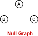
In best case: the given graph would have a null graph with no edges. So O(|V| + |E|) = O(|V| + |1|) = O(|V|) .
In average case, the given graph is moderately sparse. So, O(|E|) = O(|V|).
Therefore, O(|V| + |E|) = O(|V| + |V|) = O(|V|)
In worst case, given graph is dense. So, O(|E|) = O(|V2|) .
Therefore, O(|V| + |E|) = O(|V| + |V2|) = O(|V2|) .
-
Time Complexity of BFS = O(|V|2), if the graph is implemented using Adjacency Matrix.
If your graph is implemented as an adjacency matrix (a V x V array), then, for each node, you have to traverse an entire row of length V in the matrix to discover all its outgoing edges. Please note that each row in an adjacency matrix corresponds to a node in the graph, and the said row stores information about edges stemming from the node. So, the complexity of BFS is O(V * V) = O(V^2).
branching factor
and distance between source and destination
measured in number of edge traversals.If b = branching factor, and d = depth of the tree or graph from source to destination,
time complexity of BFS = O(bd)
Space Complexity:
We store all nodes level by level in queue starting from source node until we find the destination node or have searched all nodes reachable from source.
Space Complexity: O(|V|), where |V| = total number of nodes in the graph.
Since, O(|V|) = O(bd)
Space Complexity = O(bd), where b = branching factor, d = depth of tree or graph between source and destination.
         Give it a little thought and you would realize that
         the BFS path between source and destination
         is also the shortest path between source and destination.
BFS vs. DFS:
BFS stores all the nodes level by level (till they are processed). For an average graph this might mean requiring larger space compared to DFS. BFS uses a larger amount of memory because it expands all children of a vertex and keeps them in memory.
BFS is going to use more memory depending on the branching factor.
Space complexity of BFS is O((branching factor) ^ (distance from source to destination)) as we have seen above.
If a graph is super wide and the goal state is not guaranteed to be closer to the start node then we need to think twice before performing a BFS, since that might not give optimal result.
BFS is better when target is closer to Source (like, looking for first degree and second degree connections in Facebook Friends network, or LinkedIn Connection Network). DFS is better when target is far from source (example: DFS is suitable for decision tree used in puzzle games).
If you know a solution is not far from the start node, BFS would be better in most cases.
If solutions are located deep in the tree or graph, BFS could be impractical.
If you are looking to learn more about Breadth First Search, please take a look at
TWO END BFS.
Problem Solving:
As always, we will now do some problem solving to show you how you could solve real-world problem using Breadth First Search. We would start with a rather advanced level problem to show you the potential of BFS.
Word Break:
Given a string s and a dictionary of strings wordDict, return true if s can be segmented into a space-separated sequence of one or more dictionary words.
Note that the same word in the dictionary may be reused multiple times in the segmentation.
Example 1:
Input: s = "applepenapple", wordDict = ["apple","pen"]
Output: true
Explanation: Return true because "applepenapple" can be segmented as "apple pen apple".
Note that you are allowed to reuse a dictionary word.
Example 2:
Input: s = "catsandog", wordDict = ["cats","dog","sand","and","cat"]
Output: false
Solution:
Looking at the problem for the first time you might not even possibly imagine that this problem could be solved using BFS, unless you are already really good at Graph Theory and could quickly spot how a problem could be represented using graph. This is the beauty of this problem, and if you are a beginner I want to discuss this kind of problems with you early on so that you could realize the subtle use of graph and the huge potential and applications of Graph Theory. As always, irrespective of your current level, my goal is to eventually make you an advanced level problem solver using the concept we are currently learning.
Now back to our solution for this problem.
If a given string can be segmented into a space-separated sequence of one or more dictionary words then it would look something like below.
Input: s = "applepenapple", wordDict = ["apple","pen"]
"applepenapple" could be segmented as "apple" - "pen" - "apple".
We could restructure the segmentation and represent as below:
"apple"
       \
        "pen"
            \
             "apple"
It almost looks a root to leaf path in a graph (or, tree, to be more precise for this case), right ?
We could restructure further and represent as below:
 a
 |
 p
 |
 p
 |
 l
 |
 e
  \
   \
    p
    |
    e
    |
    n
     \
      \
       a
       |
       p
       |
       p
       |
       l
       |
       e
From above we could see that the whole string (the given string) could be represented as graph and starting from the first character we would look for substring matching any dictionary word. For each of matching dictionary words found, we would search the rest of the word (given word) starting from the character which is next to the end character of the found dictionary word (for example, if s[0...i] is a dictionary word then start searching from index (i + 1) to index (n - 1) of s where s[0...(n - 1)] is the given word).
If in our search we see that we found a dictionary word that ended at the character at the end index in the given string and the prefix before the last found dictionary word was also segmented in dictionary words, then we would know that the entire given string could be segmented in space separated dictionary words.
We could achieve this doing Breadth First Search as shown in below code. I have explained the algorithm in the inline comment in the code below.
Java code:
Login to Access Content
Python code:
Login to Access Content
Time Complexity:
O(N2), since for each of O(N) indices we search O(N) indices in the immediate suffix. N = length of the given string. Remember that we do not search an already visited suffix.
Space Complexity:
O(N). N = length of the given string.
The queue would not have more than N indices at any point of time since we do not store an already visited index again in the queue.
We would now solve an actual real-world problem:
Web Crawling.
Web Crawling:
A Web crawler, sometimes called a spider or spiderbot and often shortened to crawler, is an Internet bot that systematically browses the World Wide Web, typically operated by search engines for the purpose of Web indexing (web spidering).
The whole web could be represented using a graph, where each url would be vertex and there would be a directed edge from url A to url B if web content of url A contains (i.e, points to) url B.
In order to crawl web we should start from the starting url, read the html content for the url and discover all the urls found in the html content. Now repeat the same thing for all the discovered urls.
Now a very important thing to consider: we cannot just go on crawling forever. The Indexed World Wide Web (The Internet) contains at least 5.27 billion web pages as of Wednesday, 31 March, 2021. So the depths of the paths in the graph representing WWW from root (url from where web crawling is started) to the leaves could be very huge. If we are not interested in discovering all the web pages out there:
-
we should use BFS and not DFS, because we might be interested more in discovering the
nodes (web pages / links / urls) which are closer to the root (starting web page). Think
of it as how we are more interested in discovering first degree and second degree connections
compared to the higher degree ones.
Since DFS goes deeper till it reaches leaf and is forced to backtrack, by using DFS we would discover higher degree connections first, before discovering all the lower degree connections.
Since BFS is a level order search (searches level by level) we would discover lower order connections first. - we should have a termination condition so that we know when to stop crawling if the crawling takes a long time.
Enjoy building a simple web crawler as shown in code below. Don't forget to run the code in your local machine and play around with it, and learn as much as possible from it.
Login to Access Content
To learn about a bit more advanced Web Crawler, take a look at Multithreaded Web Crawler.
Some Amazing Applications of BFS:
- Topological Sort
- 4 Ways to Finding Cycles
- All Paths Between Two Nodes
- Bipartite Graph
- Binary Tree (De)Serialization
- N-Ary Tree (De)Serialization